Position sizing within a portfolio is an important component of managing risk. In order to avoid excessive exposure to the performance of any one stock, investors will limit the weight of stocks within the portfolio. It is not uncommon to invest, at least initially, equal amounts into each stock of a portfolio. Thereafter, the portfolio might be rebalanced periodically.
Suppose an investor has placed 2% of his nest egg into each of 50 stocks. If one company goes completely out of business and the stock drops to zero, the portfolio has only lost 2%. However, for more active investors who wish to purchase additional shares of only those stocks with the highest expected returns, maintaining an equally weighted portfolio becomes impractical; every time he wishes to add to one position, the same amount (give or take) must be added to the others.
This is undesirable, imperfect, unfortunate, indiscriminate.
Lifting Weights
An equally weighted portfolio is such that if there are N stocks in a portfolio, the desired weight of each stock is the average weight, or 1/N. In order to invest more into a stock with higher expected returns than other stocks in the portfolio, it is necessary to exceed the average weight of 1/N. If you want to get stronger, you have to lift weights. Yet, in order to limit our exposure to the performance of any one stock, it makes sense to establish a cap, C, expressed as a multiple of 1/N.
Let C/N be the maximum weight allowed for any one stock position in the portfolio, where 1 ≤ C ≤ N. For example, C = 2 means the weight of any one stock position is capped at twice the average weight. An investor who has a portfolio of 30 stocks and limits the largest position to no more than 10% of the portfolio has C/N = .10, or C = .1 x 30 = 3.
Unfortunately, within the context of position sizing, exposure or concentration risk is not addressed solely by limiting the size of any one position, but by limiting the overall combined weight of any number of positions.
For instance, suppose an investor with a 30-stock portfolio ceases investing in a particular stock when it first represents 10% of his portfolio. Now, any additional investments must go to another holding, but how much can be invested into a second stock without inviting too much exposure? Can he boost a second position up to 10% of the portfolio? Absolutely, but this cannot be done indefinitely; there could only ever be 10 stocks with such a weight. Of course, if 10 stocks comprise 100% of the portfolio, one does not have a portfolio of 30 stocks anymore. More realistically, if even just 5 of the 30 stocks were to reach 10%, they would represent 50% of the portfolio. Might this be too concentrated? Perhaps we can mathematically develop some guidance.
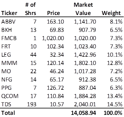
Let us suppose there are N stocks in a portfolio. The market value of a stock position in the portfolio is the number of shares held times the last closing price of the stock at a particular point in time. The weight of each stock in an N-stock portfolio can be determined by dividing its market value by the market value of the entire portfolio. Here is the Royal Dividends portfolio as of market close, December 23, 2022:
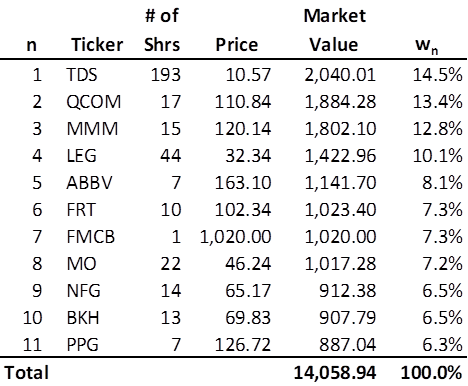
Let us rank the stocks in descending order, i.e. from most heavily weighted to the least heavily weighted. Let wn be the weight of the nth most heavily weighted stock, where n = 1, 2, . . . , N. Thus, w1 is the weight of the single most heavily weighted stock, w2 is the weight of the second most heavily weighted stock, and so forth. Lastly, wN would be the weight of the least weighted stock. Again, let’s see what this looks like for the Royal Dividends portfolio:
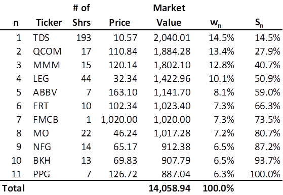
We define Sn as the sum of the weights of the n most heavily weighted stocks:

Therefore, S1 = w1, and is simply the weight of the most heavily weighted stock in the portfolio. S2 = w1 + w2, and is the sum of the weights of the two most heavily weighted stocks in the portfolio and so forth. Further, SN = w1 + w2 + . . . + wN, is the sum of the weights of all the stocks in the portfolio. It should be obvious that SN = 1 or 100%.
Indecent Exposure
Let us define Mn as the maximum weight allowance for the n most heavily weighted stocks. Thus, M1 is the maximum weight allowance for the most heavily weighted stock. This is equivalent to the maximum weight allowed for any one stock position in the portfolio. Therefore, M1 = C/N. Accordingly, we want w1 = S1 ≤ M1 = C/N. In the interest of extending the idea of mitigating exposure or concentration risk beyond capping any one stock position at a weight of M1, we seek to define Mn so that Sn ≤ Mn for n = 1, 2, . . . , N.
Now, M2 is the maximum weight allowance for the two most heavily weighted stocks. By extension, we desire S2 ≤ M2. M2 is still undefined. Should M2 = 2M1? Practically speaking, it could be. However, we know that SN = 1 and by definition SN ≤ MN. Therefore, for a fully invested portfolio, it would make sense to set MN = 1. After all, if the combined weight of all the stocks in a fully invested portfolio is always 1 or 100%, then certainly the maximum weight allowable is 1 or 100%. As we shall see, this has an interesting implication.
As n increases from 1 to N, the average weight implied by Mn goes from C/N to 1/N. This suggests that while Mn should strictly increase with n, it should do so at a declining rate. Otherwise, we wind up with the situation described earlier, where a 30-stock portfolio effectively shrinks to a 10-stock portfolio (the 20 least weighted stocks would be a negligible component, if not completely dropped from the portfolio). So while, it isn’t particularly harmful to set M2 = 2M1, doing so would mean that the implied average weight of the two most heavily weighted stocks should be capped at [2(C/N)]/2 = C/N. In going from M1 to M2, we’ve increased n by 1, but have not moved toward the 1/N average weight implied by MN. Logically, M2 should be set so that M1 < M2 < 2M1. For example, if an investor has a 30-stock portfolio and desires that no single position be greater than 10%, it would be prudent to make sure that no two stocks (and practically, the two most heavily weighted) breach X% where X is certainly greater than 10% but perhaps a little less than 20%.
The Portfolio for the Ages at Royal Dividends currently has 11 stocks and will not acquire shares of a stock if doing so would exceed a weight of 27.3%. In other words, Royal Dividends has C = 3, and thus M1 = C/N = 3/11 = .273 or 27.3%. As of market close on December 23, 2022, the most heavily weighted stock, TDS, is well under that threshold.
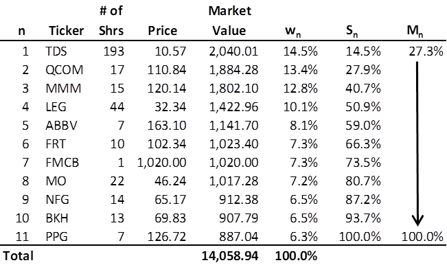
The first four stocks have received multiple additional investments over several months and now represent just over 50% of the portfolio. Might this be too much concentration? After all, this portfolio started out with a near equal share in all 11 stocks. Given the decision to have C = 3, and thus allow more than a quarter of the portfolio to rest with one company, it is likely not a problem that 4 stocks are slightly more than 50%. However, it would be useful to determine a useful, strictly increasing mathematical function of C, N, and n.
Developing a Formula
Step 1: As the Crow Flies
To begin, let’s take a closer look at a similarly sized, but equally weighted, portfolio with C = 3.
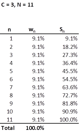
With an equally weighted portfolio of 11 stocks, the cumulative sum of the weights Sn, cannot really stand as a proxy for Mn because M1 = 3S1, allowing for a considerable overweighting of a stock. However, if one were to graph the line of Sn for n = 1, 2, . . ., 11, it is not difficult to see that it is a straight line with Sn rising by 9.1% with each n. This is a useful observation and applying the same linear characteristic to Mn produces the following:
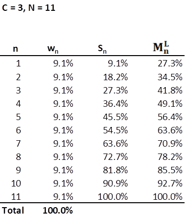
This would work in a pinch. Mn is linearly increasing by approximately 7.3% with each increase in n. M2 = 34.5% means that the implied average of the weights of the two most heavily weighted stocks is approximately 17.2%. So, there is some flexibility in overweighting multiple stocks, so long as the highest weighted stock is less than M1. For instance, if w1 = 20%, w2 = 14.5% and the remaining stocks all at 7.3%, Sn ≤ Mn for all n. However, if an investor were to max out the weight of his most heavily weighted stock at 27.3%, all the remaining stocks in the portfolio would be capped at a weight of 7.3%. So, with this definition of Mn, maxing out just one stock position means that all the remaining stock positions would have to be lower than what they would be in an equally weighted portfolio.
Put another way, if an investor is willing to triple weight one stock, so much so that it represents more than a quarter of the portfolio, does it make sense that the next holding cannot exceed 7.3%? What if two or more current holdings represent particularly good bargains with very high expected future returns? Perhaps we can allow more flexibility for overweighting multiple stocks without accepting too much risk. A linearly defined Mn is a bit restrictive in this regard so we will move on. However, the formula for a linear Mn is worth revealing and will become useful later on.
Given C, N, and n as defined above a linear Mn for n = 1, 2, . . . , N is defined thusly:

A quick glance shows M1 = C/N and MN = 1. Have a blast and test out another n or two.
Step 2: Growth? At What Cost?
Excel features the ability to fill in a trend via a ‘growth’ factor. I wondered how this might define Mn between C/N and 1. Perhaps it would rise more quickly than a linear approach and then taper off as n approaches N. Here’s how it played out:
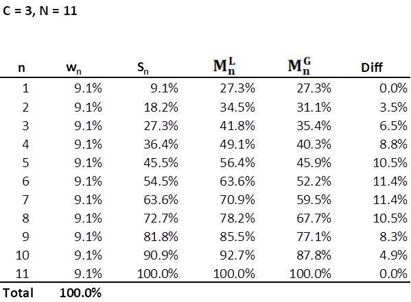
Here, the growth Mn grows by a constant multiplicative factor of 1.1387 as n increases. However, the results are impractical. Not only have we gained no flexibility over the linear Mn, even an equally weighted portfolio would fail the requirement that Sn ≤ Mn for all n. The difference of the linear over the growth is shown. Again, though this growth approach is of no use directly, the formula will come in handy later.
Given C, N, and n as defined above a growth Mn for n = 1, 2, . . . , N is defined:

Again, it is easy to see that M1 = C/N and MN = 1. If you’re bored, try some other values of n.
Step 3: Learning from Our Failures
Let us examine a graph of what we have so far.
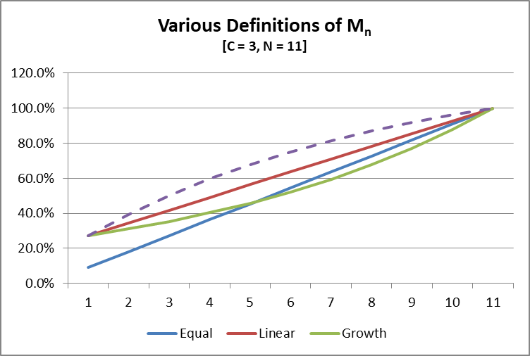
Here we can visualize that the linear approach for Mn would be adequate in monitoring a portfolio to ensure Sn ≤ Mn for all n; its line is always above the theoretical Sn = Mn of an equally weighted portfolio on which one would apply a cap, C = 3. And though the growth line is impractical, it does have one feature that we’re interested in. It bends, but not in the desired direction. The curve is convex. Imagine though, if you could flip it over the red line. I’ve depicted a dashed line that would bend in an optimal way. It would be concave and still satisfy all the desired properties.
If I still had all of my mathematical wits about me, this might have been a simple exercise without having to travel through this process. In my mind, there might have been a time in my life where I could have crafted the appropriate formula, more or less directly. Then again, maybe not. I think it is important to see the process I went through and so now we take the last step and build the formula that produces the dashed line above.
Step 4: Making Lemonade
There is an adjustment that needs to be made. The growth function is such that is grows by larger and larger absolute amounts as n increases. Thus, the increase from n = N – 1 to n = N is larger than from n = 1 to n = 2. I would rather the opposite be the case. I would like the curve of Mn to increase, but by less and less as n increases. In the table below, I reversed the order of the differences between the linear and growth columns. And where the growth curve falls under the linear by these differences, the right-most column adds these differences (in a reverse order) back to the linear column.
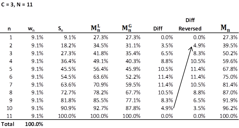
Here is the updated graph.
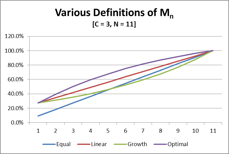
The optimal line is aptly named.
Step 5: Putting it All Together
Now, rather than build this chart for all sorts of combinations of C and N, let us construct the formula. For those of you keeping score at home, at a very high level we have:

The terms in blue allow us to add the difference between the linear and growth terms in the reversed order. So, instead of n = 2, we have n = N – (2 – 1) = N – 1. And when n = 3 we want n = N – (3 – 1) = N – 2 and so forth. Let’s fill in the details:

Simplifying:


And finally, re-writing to make the formula a bit more intuitive:

Certainly, we still have that M1 = C/N and MN = 1. The term in brackets increases at a declining rate. Thus, we start with C/N and add smaller and smaller amounts until we reach 100%.
Refining the Formula
Here is how the Royal Dividends portfolio measures up as of December 23, 2022:
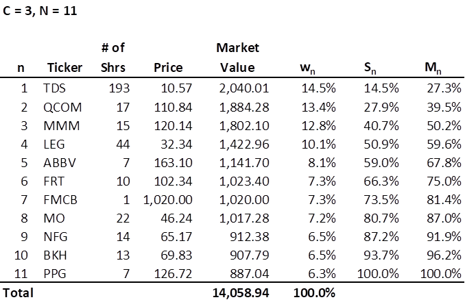
The benefits of having a formula are significant. We can immediately derive guidelines for any size portfolio paired with different caps. For instance, if an investor has a portfolio of 30 stocks and does not wish for any stock to exceed a weight of 10%, we have the following:
M1 = C/N = .10
M2 = .10 + 1 – .10(1/29) = .176
M3 = .10 + 1 – .10(2/29) = .247
M4 = .10 + 1 – .10(3/29) = .312
And so forth. The investor now knows that if the three most heavily weighted stocks exceed 25% of the portfolio, he might consider ceasing additional investment or rebalancing. Or if the four most heavily weighted stocks make up a third of the portfolio, he might be overexposed to those four stocks, even if none are over 10%.
How about an investor with 30 stocks and the desire to cap any stock at just twice the level of an otherwise equally weighted portfolio?
M1 = 2/30 = .067
M2 = .067 + 1 – .067(1/29) = .156
M3 = .067 + 1 – .067(2/29) = .237
M4 = .067 + 1 – .067(3/29) = .311
Wait, what happened here? M2 > 2M1, M3 > 3M1, etc. This would suggest that the investor would be happy with more than one stock exceeding his weight rule for one stock. This will happen when the number of stocks in the portfolio is rather large relative to the cap being put in place. This is easily solved by capping Mn by n(C/N). We present the formal definition, with no further adjustments.
In order to limit concentration or exposure risk to any subset of stocks, their combined weight should be capped at the maximum weight allowance for the n most heavily weighted stocks in an N-stock portfolio, defined for n = 1, 2, . . . , N as

where C is chosen such that 1 ≤ C ≤ N and C/N is the maximum weight allowance for any one stock position.
Let us revisit the investor with a 30-stock portfolio and a desire to limit any one position from attaining a weight of twice that of the average weight (i.e., C = 2). This time, we will use the full definition of Mn.
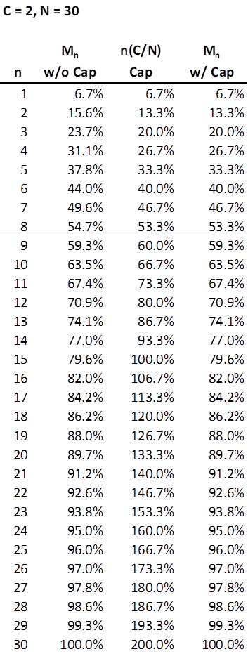
Setting C = 2 for a portfolio with 30 stocks means that no stock weight can exceed 6.7%. That’s a fairly low cap for a portfolio of this size. So, though the investor cannot place as much as say 10% in any one position, he can have as many as 8 stocks representing just over 53% of the portfolio (provided the remaining 22 stocks are collectively, minimally weighted), before breaching his own theoretical tolerance for exposure risk. Beyond n = 8, the minimum of n(C/N) is no longer applicable.
The graph that follows depicts the capping effect on Mn for n = 1 through 8. Note that from n =15 through n = 30, the n(C/N) cap becomes nonsensical, exceeding 100%. The y-axis has been truncated at 100% to better illuminate the impact of the cap when it does apply.
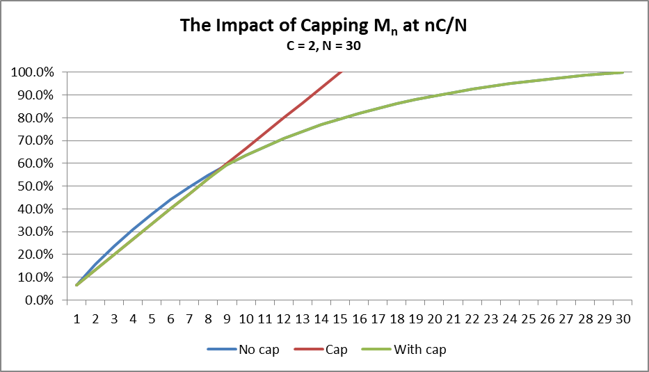
The green line representing Mn with its cap in place, is linear up through n = 8 and then concave upward from that point as designed.
Using the Formula
There is something rather intuitive about this definition for Mn. Clearly, if an investor sets a cap of C times the portfolio’s average weight, then no stock’s weight should be allowed to exceed C/N and by definition, Mn ≤ nC/N for all n. In other words, if Mn > nC/N, that is, if the maximum weight allowance for the n most heavily weighted stocks is set to be greater than n times the maximum weight allowance for a single stock, then at least one stock’s weight would be allowed to exceed C/N – a contradiction. Thus having n(C/N) as a minimum makes perfect sense and is a given. However, what seems intuitive and what should be appealing to an investor is the idea that C/N plays a critical part of the formula.
Setting C relative to the number of stocks chosen for the portfolio implicitly defines the investor’s risk tolerance, at least with regard to position size. M1 = C/N is easy for an investor to understand, communicate, and monitor. Using this ratio to build out an equivalent guideline for an investor’s n most heavily weighted stocks seems only natural. Having the capacity to generate the totality of this array of weight thresholds in a simple mathematical formula with readily available variables C, N, and n, allows the investor a quick means of checking whether or not a subset of his most heavily weighted stocks is still within his own risk tolerance, particularly when he has not yet reached the maximum weight allowance for any single stock.
There is even an intuitive relationship between C and N. Larger portfolios can handle larger Cs. For instance, setting C = 2, when N = 50 prevents significantly overweighting a stock. Each number actually speaks to the investor’s risk tolerance. Assuming there is balance among the sectors within the 50-stock portfolio, one could argue that just having that many stocks is a sign that the investor’s risk tolerance is not high. Full diversity is achieved at a much lower level. Capping any one position at just 4% of the entire portfolio is another indication of a lower level of risk tolerance. There is absolutely nothing wrong with this. If, however, the investor has a strong conviction about the expected future returns of even just one company, his or her hands are a bit tied. With careful management, the investor could push as many as 8 stocks to the max, but it isn’t often the case that an investor has so many promising choices for additional investment. More often the best avenues of additional investment are limited to just a handful of stocks, in even the largest portfolios. A 50-stock portfolio can more readily accept a C as high as 4 or 5, than significantly smaller portfolios.
I am a long-time subscriber of the excellent Sure Dividend Newsletter, and a portion of my assets has been dedicated to following every trade of their Real Money Portfolio which began in January 2019. That portfolio now has 30 positions and additional funds are added periodically to existing positions up to 10% of the portfolio’s value. I used this 10% cap within the context of a 30-stock portfolio (which implies C=3) as inspiration for having a similar constraint within the 11-stock Royal Dividends portfolio. Here, C=3 on a portfolio of just 11 holdings allows the weight for any one stock to be substantially higher.
It may seem a bit aggressive to have M1 = 27.3%, but consider the following four points: (1) if one is willing to have (at least initially) just 11 stocks represent their foray into the world of equities, they’re already comfortable with risk, (2) risk is not managed by position size alone; all but two stocks in the current portfolio are Dividend Kings, and there is exposure to every sector as well, (3) eventually, with the passage of enough time, none of the current holdings will be considered among the Top Ten stocks with the highest expected returns, and a new position will be added, effectively increasing N and lowering M1, and (4) one can always change their risk tolerance.
Lastly, the mathematics above could be modified to aid one in monitoring weights across sectors or industries, etc. That’s a discussion for another post – hopefully, written by someone else.
