If you look up summary data on a given ticker symbol on a broker’s webpage or say, Yahoo! Finance, you’ll encounter various statistics on the price, price ranges, volumes, earnings, outstanding shares, dividends, etc. Here’s a look at the summary data for American States Water [AWR] on Yahoo! Finance, after trading hours on August 9, 2022.
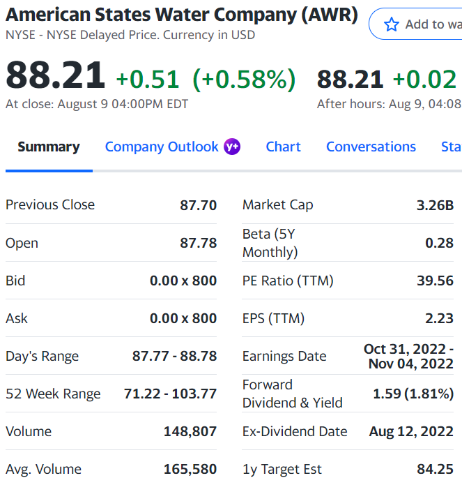
Most of these are either self-explanatory or easily understood with context. There is one item, however, that offers no real clues as to what it is and what it says about the stock you’re looking at: Beta.
A Definition of Beta
Here is TD Ameritrade’s definition of beta:
The measure of a security’s volatility in relation to the S&P 500. Beta less than 1 means the security’s price or NAV has been less volatile than the market. Beta greater than 1 means the security’s price or NAV has been more volatile than the market.
Royal Dividends is not concerned with mutual funds, so let’s ignore the mention of NAV or net asset value. Beta measures the responsiveness of a stock’s price to changes in the overall stock market. For a U.S. equity, the S&P 500 is used as a proxy for the entire market. Plenty of internet sources go even further with their definition, suggesting that beta can be used to create expectations about the future performance of a stock. Typically, they’ll provide an example like this: if the S&P 500 were to move up 10%, a stock with a beta of 1.5 could be expected to move up 15% (1.5 x 10). Likewise, if the market is due for a 10% correction, we could expect that same stock to drop 15%.
I don’t recommend forming expectations of return based on beta. First, beta is a rearview look. The future will be different. Second, it is a single-number summary of a multitude of data points. It’s the equivalent of saying the average temperature in Syracuse this past year was 55 degrees. Just as dressing for that temperature will leave you freezing 7 months of the year and sweating the other 5 months, expecting a stock to return 1.5 times the market’s return for a particular month, just because it has a beta of 1.5, is a bad idea.
Raw Data
To better understand beta we need to see how it is calculated at least once. Neither TD Ameritrade nor Yahoo! Finance provide the specifics of how they calculate beta. However, the latter does provide two clues when they say Beta (5Y Monthly). This means Yahoo! calculates beta looking at monthly returns over a 5-year lookback period, a total of 60 data points.

Yahoo! Finance allows an individual to download historical prices to facilitate spreadsheet analysis. I chose to download monthly data going back 61 months so that I can get the last 60 months of returns. GSPC is the ticker symbol they use for the S&P 500. I isolated the unadjusted closing price for each calendar month from the half-dozen or so fields I received in the download. Ultimately, it proved to be the correct field to tie back to their beta calculation.
Just looking at the monthly returns of the index and AWR, one can see considerable volatility in each and while there are some similar moves, there are plenty of differences in direction and magnitude. Beta is a single numerical representation of this 5-year period. How do we boil it down to one number?
Calculating Beta
There are five ways to calculate beta in Excel. All five give you exactly the same answer. I present these methods in order of decreasing complexity, until Method 5, which is a visual approach. But as Don Lapre used to say, “Choose the one that excites you the most.”
Method 1
This method is not for the faint of heart. I have to put it in here, because math and statistics are divine.

It is easier than it looks to make the table above. The symbols are just for fun. The first three columns you’ve already seen. They’re the months and the monthly returns for the S&P 500 and AWR, this time shown as decimals and not as percentages for appearance purposes only. The index monthly returns is our independent variable X. AWR’s monthly returns are the dependent variable Y, because in theory some of the variation in returns is derived from that of the index. The next two columns are the deviations of those returns from their averages (x̅ and y̅ respectively) which are shown in the box below the return columns 2 and 3.
The second to last column is the product of columns 4 and 5. The last column is column 4, squared. The ratio of the sums of those last two columns (column 4 divided by column 5) makes beta (shown in its Greek beauty). It ties to the Yahoo! Finance figure. TD Ameritrade only displays beta to the tenths decimal place and has AWR with a beta of .3. I’ve checked a few companies; I have every reason to believe they’re doing exactly the same calculation and simply rounding it.
Method 2
This method involves installing the ‘Analysis Tool Pak’ add-in through the Excel Options menu and then finding ‘Regression’ (upon relaunching Excel) under the ‘Data Analysis’ menu of the ‘Data’ tab. Click on ‘Regression’ and highlight the stock returns for the Y-range and the index returns for the X-range. Click ‘OK’ and you get the following information on a new worksheet.
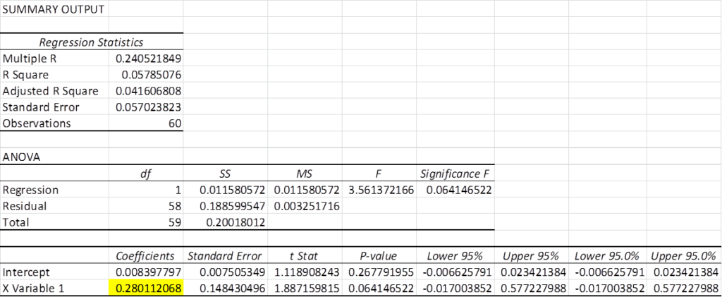
It’s a lot of information if you’re just interested in beta. Beta is the X-coefficient in a standard linear regression, which is what we just conducted. Essentially, you just ran a macro that built the table from Method 1 behind the scenes.
Method 3
If you have no need for the abundance of statistical information in the regression routine, use this method.
Enter the following formula into a blank cell:
=COVARIANCE.P(stock return range, index return range)/VAR.P(index return range)
Now, for the love of God, don’t type ‘stock return range’ and ‘index return range’. Input the actual ranges of your data. Order doesn’t matter in the numerator, but the index returns need to be in the denominator. You’ll get the same answer yet again. This formula is interesting in that it sort of describes what it is you’re doing when you examine beta. You’re assessing how the stock varies with the index, relative to the variability of the index itself.
Method 4
The regression routine refers to beta as the coefficient of the independent variable X. It is also the slope of the best-fitting, linear regression line. We’ll get to that shortly. In the meantime, try the following formula and you’ll get the exact same answer as the other methods.
=SLOPE(stock return range, index return range)
Now, order matters here; the dependent variable (the stock’s returns) must be first. This formula is just a little easier to enter and so it is my favorite.
Method 5
This method relies more on chart building skills, and it is the most beautiful. I’ll be brief, because I don’t want to make this an Excel tutorial. Essentially, if you highlight the two return ranges, with your stock on the right, and choose to insert a ‘Scatter’ plot chart (the first one, because it does not depend on the monthly order of the X-values), you get a scatter plot. Then you can opt to show a linear trend line and its formula. The formula reveals the correct beta value as the coefficient of X. Now, the chart won’t look as nice as the one below. I took the time to format it, because formatting is even more important than the accuracy of the calculations. Would you even get far enough to question accuracy, if you’re repulsed by the graph? On the subject of formatting, here is one of my favorite quotes, an excerpt from Benjamin Franklin’s autobiography (referring to his growing printing business):
Bradford still printed the votes and laws and other public business. He had printed an address of the House to the governor, in a coarse, blundering manner; we reprinted it elegantly and correctly, and sent one to every member. They were sensible of the difference; it strengthened the hands of our friends in the House, and they voted us their printers for the year ensuing.
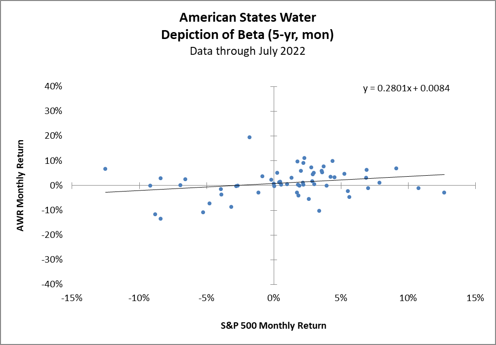
So long as the two returns for each month are always paired together, the month order is not important to the calculation of beta. And just so you know what it is you’re looking at, the left-most dot represents March 2020, when the market returned -12.5% and American States Water returned 6.7%. It turns out, Covid did not change our need for water. The right-most dot on the graph is the very next month April 2020. The market returned 12.7% and AWR returned -2.9%. Apparently, we were just a bit too excited about water.
A Picture is Worth a 1,000 Words
Unfortunately, sometimes those words are in a foreign language. As you’ll come to find out in subsequent posts on beta, just knowing how to calculate it or what it represents visually doesn’t really lend clarity to how it can be used to your advantage. The scatter plot of the paired returns is, with its best-fitting, linear regression line is a wonderful way to picture beta. Beta is the slope of that line.
Here’s the scatter plot for H.B. Fuller Company. Their beta of 1.57 is the highest among the Dividend Kings.
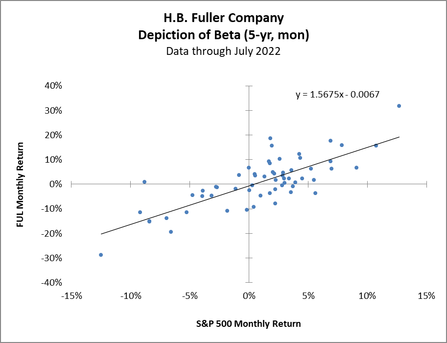
The beta is higher for FUL and so the slope is greater. Is a higher beta better? Nope. There are option trading strategies that do seek out, and benefit from, higher beta stocks because their options premiums are higher. Others buy high beta momentum stocks in the hopes they take off with the next strong, upward move in the market. Unfortunately, while a stock’s returns are used in the calculation, one cannot discern anything about the stock’s return over the period from beta. That might ultimately be the most intuitive reason as to why beta shouldn’t be used for building return expectations. If one can’t discern the historical return over the period on which the beta is based, why should we think it would be any more reliable for predictions of the future?
H.B. Fuller’s annualized price appreciation (ignoring dividends) over the 60 months was 4.5%, quite a bit lower than that of the S&P 500’s annualized return of 10.8%. American States Water, with its much lower beta of .28, outperformed the market with an annualized return of 12%, again not taking dividends into account.
Are you curious as to which Dividend King has the lowest beta? Do you like Tootsie Rolls?
Who Doesn’t Like a Tootsie Roll?
Tootsie Rolls Industries Inc [TR] has a beta of -.01 and is the only King with a negative beta.
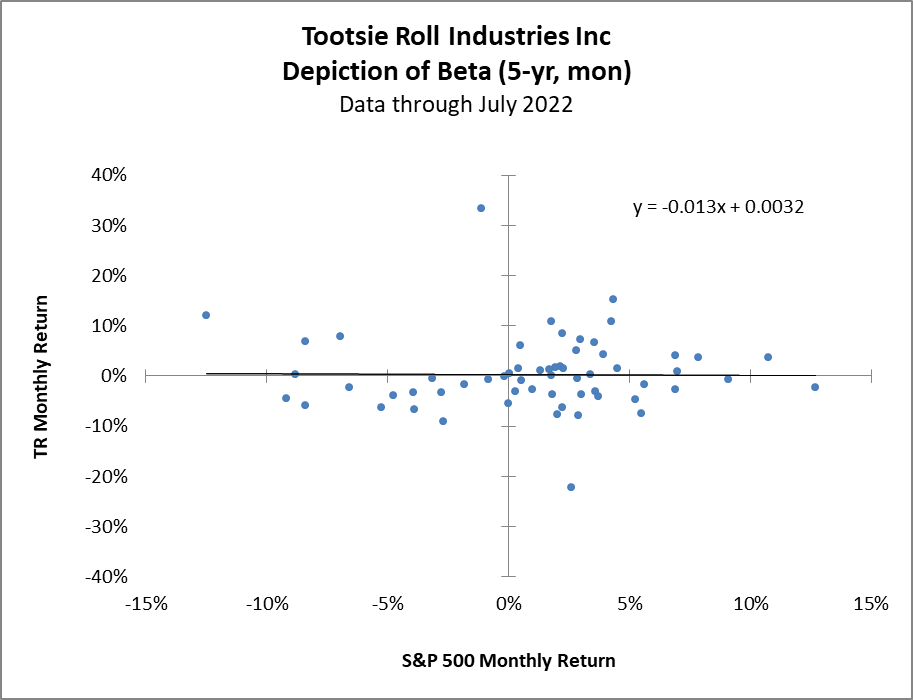
The linear regression line is barely distinguishable from the x-axis, but it’s there, and it is actually sloping down to the right. TR’s average annual return (excluding dividends) was 0.6%.
Part 2 of this discussion on beta will try to further destroy the notion that there exists a practical application of beta to boost returns.
